
I got the idea to make a wave simulator, and after some research found out about the discretized wave equation, which uses a finite difference approximation of the actual wave equation.
Using the macroquad crate, I was able to throw together a simple CPU based simulator in about an hour, but even at the small resolution of 720 by 406, I was only getting about 30 FPS.
I have wanted to make a project that deals with the GPU for months now, and this was just the perfect project for GPU acceleration because each pixel is updated independently of the others every time step, so we can take advantage of the massive parallelization of GPUs to render much faster. (About 7000 updates per second on my RTX-2080!)
Keep scrolling for more cool images and videos! (Or just click here to skip)
The Discretization
I did not derive the approximation myself, I found it in a great YouTube video from Nils Berglund, “Tutorial: How to simulate the wave equation”. Note that there is a typo in the video and the discretized equation incorrectly drops the square on , which would end up being a pain to debug later on. The original partial derivative for the wave equation and the discretized version are below.
In these equations, and are the pixel coordinates, and are the time step, and is the Courant number, which is a dimensionless quantity the incorporates the medium’s wave speed, the time step, and the length interval (size of each pixel).
Implementing this equation in code is actually fairly straightforward, the hardest part being that you have to juggle some buffers around to avoid reallocating. Here is my final implementation in WGSL (WGPU Shader Language):
next_states[i] = 2.0 * states[i]
    - last_states[i]
    + pow(ctx.c, 2.0) * (
        states[index(x - 1, y)]
        + states[index(x + 1, y)]
        + states[index(x, y - 1)]
        + states[index(x, y + 1)]
        - 4.0 * states[i]
    );
Running on the GPU
This was my first project that really deals with the GPU, so I was completely new to most of this. All I knew is that I wanted to use wgpu and that the calculations should be done in a compute shader. If you don’t know, wgpu is a rust implantation of the WebGPU standard that basically abstracts over low level graphics APIs like OpenGL, Vulken, Direct3D, and Metal. Compute shaders basically just run code for arbitrary “work units” rather than for every vertex in the scene or pixel on the screen.
All things considered, the GPU implementation was actually kinda easy. In only about 150 lines of rust, I was able to load my shader code and repeatably dispatch it to run. By just passing the buffers to the shader in a rotating order every frame, everything just worked. Only problem being that I couldn’t see anything.
@group(0) @binding(0) var<uniform> ctx: Context;

@group(0) @binding(1) var<storage, read_write> next_states: array<f32>;
@group(0) @binding(2) var<storage, read> states: array<f32>;
@group(0) @binding(3) var<storage, read> last_states: array<f32>;

struct Context {
    width: u32,
    // ...
}

fn index(x: u32, y: u32) -> u32 {
    return y * ctx.width + x;
}

@compute
@workgroup_size(8, 8, 1)
fn main(@builtin(global_invocation_id) global_id: vec3<u32>) {
    let x = global_id.x;
    let y = global_id.y;
    let i = index(x, y);

    // SNIP (Shown Above)
}
Visualizing the Simulation
After finishing the actual simulation, I thought the visualization would be easy enough. I was very wrong. After almost four hours of intense graphics programming later, I finally got it rendering to a window. Initializing the GPU and managing the compute shader took just about 150 lines of code but adding all the rendering stuff brought it up to over 400 lines. All the refactoring and random features I ended up adding later brought it over a thousand lines.
I had to create a render pipeline, vertex data, a vertex buffer, a window, create a surface (frame buffer), and finally execute the render pass after the compute shader. As someone very new to all this graphics stuff, this took a long time to figure out. But when I did, the joy I felt seeing a tiny little grayscale wave propagate across my screen was… a little sad, but whatever.
The way it works it by rendering a big quad over the whole viewport, and in the rasterization stage the fragment shader is called for each pixel, it can then index into the current state buffer and return the appropriate color. For coloring, I decided to make positive values range from white to pure blue and negative values range from white to pure red.
Here is a simplified version of the fragment shader that doesn’t deal with any of the different render modes or windows that aren’t the exact same size as the simulation. I’ve heard that if statements are bad in shaders, so I multiplied the color by the value of the condition instead of using an if statement. No idea if this is a good idea, or any faster.
@group(0) @binding(0) var<uniform> ctx: Context;
@group(0) @binding(1) var<storage, read> states: array<f32>;

struct Context {
    width: u32,
    // ...
}

@fragment
fn frag(in: VertexOutput) -> @location(0) vec4<f32> {
    let x = u32(in.position.x);
    let y = u32(in.position.y);

    let val = states[y * ctx.width + x];
    let color = (
          vec3<f32>(0.0, 0.0, 1.0) * f32(val > 0.0)
        + vec3<f32>(1.0, 0.0, 0.0) * f32(val < 0.0)
    );

    let aval = abs(val);
    return vec4<f32>(color * aval + (1 - aval), 1.0);
}
The User Interface
At this point, once simulations were started, you could play/pause them with the space bar, but otherwise there was no way to control them, so I decided to add egui. This should have been super easy, but unfortunately I messed something up with event handling so even though events were being passed to egui properly, they were being cleared before the UI rendered…
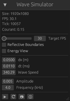
Anyway, this is the UI I currently have. At the top it shows some information like the simulation size, FPS, simulation tick, and the Courant number. Below that you can adjust some simulation settings like the target FPS, the boundary conditions, the render view, the size of each pixel and the length of each time step. Below that are the oscillator controls for amplitude and frequency. Finally, there are some buttons for play/pause, reset, screenshot, and about.
Boundary Conditions
In the previous section, you saw a toggle for “Reflective Boundary Conditions”, which are actually the easiest to implement. To implement reflections, all you have to do is ensure that the border pixels are always 0, and the reflections will happen naturally.
Absorbing boundary conditions (ABCs), the default in my program, were actually a bit of a struggle because of the previously mentioned typo in the discretized wave equation. Below is the partial derivative that defines ABCs. There are different approximations you can use for ABCs, each more accurate, however they also get significantly more complicated, so I just used the simplest one. The inaccuracies in the ABC manifest as small unwanted reflections at the boarders, but because they are so small, they are usually unnoticeable.
With some basic algebra on the first approximation, I created the following equation. Where is the time step, is the state of the current border pixel and is the neighbor of the current pixel. By setting the difference in time to c times the difference from the border pixel, we cancel most of the wave.
In the shader code, I got lazy and just used a bunch of if statements to define what direction to cancel the waves in, which I expected to have a poor effect on performance, but it didn’t actually make any change. There are some other boundary conditions, for example wrapping the screen around at the borders or allowing the borders to move with the wave, but for now I’m happy with just reflective and absorbing.
Configuration
There were lots of demos I wanted to make, but changing the code every time was getting annoying, especially because I would delete my changes to try something else then end up remaking it.
I ended up making a params.toml file for each demo.
All fields are required expect map and shader.
size = [1920, 1080]
reflective_boundary = false

map = "map.png"
shader = "shader.wgsl"

dx = 0.05
dt = 0.04

v = 340.29
amplitude = 0.03
frequency = 4.0
This file defines all the properties for the simulation, we just need to define where the emitters, walls, and value at each point. To do this there are two options, a map or a shader.
A map is an image file where the red channel is used for walls, the green channel is used for emitters, and the blue channel defines what percent of the global c value is at the position (, , ). This is good for complex shapes, for example the fresnel lens. The problem with a map is that it can’t be dynamic.
A shader is a function that is compiled with and called by the actual compute shader every frame that allows you to modify the simulation while it’s running, for example for a moving emitter, or just for dynamic sizing like with the double-slit example.
The Demos
Finally! Hopefully that information was interesting, but here is the cool stuff 😎.
Click the images to watch a video of the simulation.
The Double Slit Experiment
The classic double-slit experiment, implemented with a shader so it can be easily resized. (demo source)

Lens
A biconvex lens focusing incoming light to a point. (demo source)

A fresnel lense, also focusing light to a point, but the lens is much thinner. (demo source)

Energy View
After looking at some other wave simulators online, some of them had something called the “average energy view”, which showed the average square of the value at each pixel over each time step. I also added support for this in my simulator, and it produced some interesting results.
The basic lens.

A medium with a randomized wave speed throughout.

Two in-phase emitters.

A phased array of 15 emitters.

Conclusion
Well this was a fun little project! (feel free to give it a star on GitHub) I’m really happy to have finally started working with the GPU, I have a few more projects in mind that are now possible. No idea how difficult it would be, but compiling to WASM would be a really cool addition. I also want to experiment with piping audio through the simulation to get different effects.
It was a little surprising to me how simple the simulation was to implement. I probably spent at least a week just playing with it and making these demos afterward. If you are interested in this at all I would definitely recommend making your own simulator and playing around with it.
Have a nice day!
Links
Here are some of my wave-simulator related links that may be of interest.
- Rendering Solutions to the Wave Equation in 3D
- Project GitHub Repository
- My Original Simulation Code
Here are links to some additional resources that may be of help if you want to make your own simulation. Definitely watch Nils Berglund’s video, it was probably the most helpful resource I found.